Tweedie Distribution
For Dramatically Unbalanced & Zero-inflated Data
- Is that a typo?
- Ok… So what?
- Clarifying our use-case
- Math time: deriving the Tweedie
- Coding a Tweedie loss
Is that a typo?
The Tweedie distribution is a three-parameter family of distributions that is a special case of exponential dispersion models, but is a generalization of several familiar probability distributions, including the normal, gamma, inverse Gaussian and Poisson distributions. The distribution along with exponential dispersion models were introduced by Jørgensen in 1987.1 According to its Wikipedia page, the unusually named distribution was named as such by Jørgensen after Maurice Tweedie, a statistician and medical physicist at the University of Liverpool, UK, who presented the first thorough study of these distributions in 1984.2
Ok… So what?
You are now asking yourself; How did I come across such an oddly-named distribution, and why are you writing about it?
Well, the application of the Tweedie distribution primarily involves regression problems with an extreme class imbalance. How extreme? The majority class is at least 90% of the data. So that is really imbalanced. Having dealt with class-imbalance problems in a classification setting, I was interested in a regression use-case. But why do we need a special distribution? Couldn’t a Poisson distribution work, or even a zero-inflated hurdle model?
As it turns out, the answer to those questions is “yes, but you can do better with the Tweedie distribution.” Let’s find out why.
Clarifying our use-case
Imagine a not so far-fetched scenario were we have a cluster of data items at zero, and a right long-tailed distribution. We can clearly not fit a normal distribution to it as the data would consist of a large peak at zero and continuous positive values. Poisson is also not a suitable candidate as we are not dealing with the count data alone. On the other hand, Gamma distribution does not take zero values. This is where the Tweedie distribution shines.
This particular property makes it useful for modeling premiums in the insurance industry. Consider the properties these measures exhibit, which would need to be approximated by the probability distribution used to describe them: they are most often zero, as most policies incur no loss; where they do incur a loss, the distribution of losses tends to be highly skewed. As such, the pdf would need to have most of its mass at zero, and the remaining mass skewed to the right. This model can also be applied in other use cases across industries where you find a mixture of zeros and non-negative continuous data points.
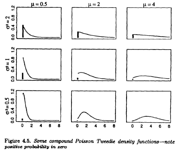
Here are some of the first illustrations of a Tweedie Distribution where p = 1.5, from one of Jørgensen’s original analyses:3

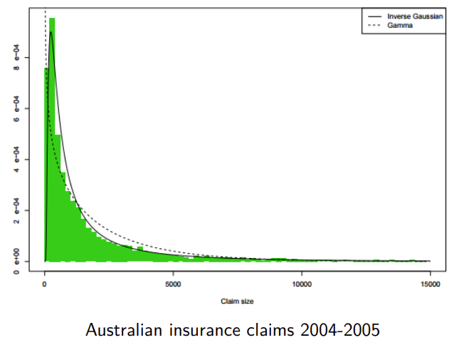
And a practical example of insurance claim payments:4

Math time: deriving the Tweedie
The Tweedie distribution has three parameters:
- mean $\mu$
- dispersion $\phi$
- power parameter $p$
The distribution is characterized by a unique mean-variance relationship $var(Y) = \phi \mu^p$. Setting p=1 gives a quasi-Poisson distribution, while p=2 gives a gamma distribution. In practice, $p$ is a float between 1 and 2, and can be optimized as a hyperparameter via grid search given the relatively small search space. Technically speaking the distribution is not defined outside of the ranges $1 < p < 2$, but when p=0, we have a normal distribution and when p=3, we have an inverse Gaussian distribution. Thus we can directly see how the Tweedie distribution combines the Poisson and Gamma distributions. Thanks to the Tweedie distribution, our choices in modeling are not restricted to the moderately-skewed gamma distribution and the extreme skewness of the inverse Gaussian. The Tweedie provides a continuum of distributions between those two by simply setting the value of p to be between 2 (gamma) and 3 (inverse Gaussian).
Again, the area of the p parameter space we are most interested in is between 1 and 2. At the two ends of that range are Poisson, which is a good distribution for modeling frequency, and gamma, which is good for modeling magnitude. Between 1 and 2, Tweedie becomes a neat combination of Poisson and gamma, which is great for modeling the combined effects. In this way the Tweedie distribution may be thought of as a “Poisson-distributed sum of gamma distributions.”5
Let $N$ be a random variable with Poisson distribution and $Z_1, Z_2, …$ be independent identically distributed random variables with Gamma distribution. Define a random variable $Z$ by
The resulting distribution of $Z$ is called a compound Poisson distribution. In the case of insurance premium prediction $ $ refers to the number of claims, $Z_i$ refers to the amount of $i$-th claim. The PDF can be written as follows:
Where $a(\cdot )$ and $\kappa(\cdot )$ are given functions.
The compound Poisson distribution is a special case of Tweedie model, if we re-parameterize the compound Poisson by
then it will have the form of a Tweedie model Tw($\mu, \phi, \rho$) with the PDF:
The log-likelihood of the PDF can be written as
where $a, \phi, \mu$ and $1<\rho < 2$ are some constants.
To convert Tweedie distribution to a loss function, we need to maximize the likelihood of sample data through model training. A common way to do this is through the negative log-likelihood. For computational stability instead of optimizing $\mu$ parameter of Tweedie distribution directly, we will optimize $\log{\mu}$ . So changing our notation a bit, the Tweedie loss is given by the following formula:
where $w_i$ are object weights, $y_i$ is target, $F(x_i)$ is current object prediction, $\rho$ is the obligatory variance power. Variance power must belong to the interval $[1, 2]$.
Coding a Tweedie loss
The loss function of Tweedie is created for the aim of maximizing the negative log likelihood of the Tweedie distribution. Lightgbm computes Tweedie loss as follows:
def tweedie_eval(y_pred, y_true, p=1.5):
    y_true = y_true.get_label()
    a = y_true*np.exp(y_pred, (1-p)) / (1-p)
    b = np.exp(y_pred, (2-p))/(2-p)
    loss = -a + b
    return loss
A Tensorflow implementation would look as follows:
import tensorflow as tf

def tweedie_loss_func(p):
    def tweedie_loglikelihood(y, y_hat):
        loss = - y * tf.pow(y_hat, 1 - p) / (1 - p) + \
               tf.pow(y_hat, 2 - p) / (2 - p)
        return tf.reduce_mean(loss)
    return tweedie_loglikelihood
Scikit-learn has an implementation of a Tweedie Regressor.6 H20 even has a gradient boosting implementation with a Tweedie distribution!7 Here is a general framework for how it can be used:
import h2o
from h2o.estimators.gbm import H2OGradientBoostingEstimator
from h2o.grid.grid_search import H2OGridSearch


gbm = H2OGradientBoostingEstimator(distribution="tweedie",
								   tweedie_power = 1.2,
								   seed =1234)

gbm.train(x = predictors,
		  y = response,
		  training_frame = train,
		  validation_frame = valid)


# Example of values to grid over for `tweedie_power`
# select the values for tweedie_power to grid over
hyper_params = {'tweedie_power': [1.2, 1.5, 1.7, 1.8]}

gbm_2 = H2OGradientBoostingEstimator(distribution = "tweedie",
									 seed = 1234,)

grid = H2OGridSearch(model = gbm_2,
					 hyper_params = hyper_params,
                     search_criteria = {'strategy': "Cartesian"})


grid.train(x = predictors,
		   y = response,
		   training_frame = train,
		   validation_frame = valid)

sorted_grid = grid.get_grid(sort_by = 'mse',
							decreasing = False)
print(sorted_grid)
And my favorite code implementation: CatBoost!
from catboost import CatBoostRegressor, Pool

train_pool = Pool(df_train[features],
				  label=df_train[target],
				  cat_features=cat_features)
test_pool = Pool(df_test[features],
				 label=df_test[target],
				 cat_features=cat_features)

cb_tweedie = CatBoostRegressor(loss_function='Tweedie:variance_power=1.9',
							   n_estimators=500,
							   silent=True)
cb_tweedie.fit(train_pool, eval_set=test_pool)
-
Jørgensen, B. (1987), Exponential Dispersion Models. Journal of the Royal Statistical Society: Series B (Methodological), 49: 127-145. https://doi.org/10.1111/j.2517-6161.1987.tb01685.x ↩
-
Tweedie, M.C.K. (1984). “An index which distinguishes between some important exponential families”. In Ghosh, J.K.; Roy, J (eds.). Statistics: Applications and New Directions. Proceedings of the Indian Statistical Institute Golden Jubilee International Conference. Calcutta: Indian Statistical Institute. pp. 579–604. MR 0786162 ↩
-
Kelly, Jorgensen (1996). Analyzing Accident Benefit Data Using Tweedie’s Compound Poisson Model. ↩
-
Heller et al. (2007) Mean and dispersion modelling for policy claims costs. ↩
-
M. Goldburd, A. Khare, D. Tevet, D. Guller (2016). Generalized linear models for insurance rating, _Casualty Actuarial Society, CAS Monographs Series. ↩
-
https://scikit-learn.org/stable/modules/generated/sklearn.linear_model.TweedieRegressor.html ↩
-
https://docs.h2o.ai/h2o/latest-stable/h2o-docs/data-science/algo-params/tweedie_power.html ↩