Bayesian Optimization
- What are hyperparameters?
- Back-box optimization
- Naive approaches for hyperparameter optimization
- Introducing Bayesian hyperparameter optimization
What are hyperparameters?
All machine learning models have a set of hyperparameters or arguments that must be specified by the practitioner. These are values that must be specified outside of the training procedure. Vanilla linear regression doesn’t have any hyperparameters. But variants of linear regression do. Ridge and Lasso Regression both add a regularization term to linear regression; the weight for the regularization term is called the regularization parameter. Decision trees have hyperparameters such as the desired depth and number of leaves in the tree. Support Vector Machines require setting a misclassification penalty term. Kernelized SVM require setting kernel parameters like the width for RBF kernels.
These types of hyperparameter control the capacity of the model, i.e., how flexible the model is, how many degrees of freedom it has in fitting the data. Proper control of model capacity can prevent overfitting, which happens when the model is too flexible, and the training process adapts too much to the training data, thereby losing predictive accuracy on new test data. So a proper setting of the hyperparameters is important.
Another type of hyperparameters comes from the training process itself. For instance, stochastic gradient descent optimization requires a learning rate or a learning schedule. Some optimization methods require a convergence threshold. Random forests and boosted decision trees require knowing the number of total trees. (Though this could also be classified as a type of regularization hyperparameter.) These also need to be set to reasonable values in order for the training process to find a good model.
Back-box optimization
Conceptually, hyperparameter tuning is an optimization task, just like model training. However, these two tasks are quite different in practice. When training a model, the quality of a proposed set of model parameters can be written as a loss function. Hyperparameter tuning is a meta-optimization task. Since the training process doesn’t set the hyperparameters, there needs to be a meta process that tunes the hyperparameters. It is a process commonly referred to as black-box optimization, meaning that we want to minimize a function $f(\theta)$ but we only get to query values rather than directly computing gradients. This is why hyperparameter tuning is harder- the quality of those hyperparameters cannot be written down in a closed-form formula, because it depends on the outcome of a blackbox (the model training process). This is why hyperparameter tuning is much harder.
Naive approaches for hyperparameter optimization
Up until a few years ago, the only available methods were grid search and random search. Grid search evaluates each possible combination, and returns the best configuration based on a loss function. Unlike grid search, a key distinction with Random search is that we do not specify a set of possible values for every hyperparameter. Instead, we sample values from a statistical distribution for each hyperparameter. A sampling distribution is defined for every hyperparameter to do a random search. In fact, in a 2012 paper Bergstra and Bengio proved that in many instances random search performs as well as grid search.1
The implementation of these methods is simple; for each proposed hyperparameter setting, the inner model training process comes up with a model for the dataset and outputs evaluation results on hold-out or cross validation datasets. After evaluating a number of hyperparameter settings, the hyperparameter tuner outputs the setting that yields the best performing model. Formally this can be represented as
Here we are minimizing the score of our evaluation functon evaluation over the validation set. $x^*$ is the set of hyperparameters that yields the lowest value of the score.
The last step is to train a new model on the entire dataset (training and validation) under the best hyperparameter setting.
Hyperparameter_tuning (training_data, validation_data, hp_list):
  hp_perf = []
  foreach hp_setting in hp_list:
    m = train_model(training_data, hp_setting)
    validation_results = eval_model(m, validation_data)
    hp_perf.append(validation_results)
  best_hp_setting = hp_list[max_index(hp_perf)]
  best_m = train_model(training_data.append(validation_data), best_hp_setting)
  return (best_hp_setting, best_m)
Grid and random search are naive yet comprehensive. However, their computational time increases exponentially with a growing parameter space. They also don’t utilize search results from previous iterations.
Introducing Bayesian hyperparameter optimization
Hyperparameter optimization has proven to be one of the most successful applications of Bayesian optimization (BO). While BO is an area of research decades old, it has seen a resurgence that coincides with the resurgence in neural networks granted new life by modern computation: the extreme cost of training these models demands efficient routines for hyperparameter tuning.
BO will allow us to answer the question; Given a set of observations of hyperparameter performance, how do we select where to observe the function next?
Big picture
At a high-level, BO methods are efficient because they choose the next hyperparameters in an informed manner. The basic idea is: spend a little more time selecting the next hyperparameters in order to make fewer calls to the objective function. In practice, the time spent selecting the next hyperparameters is inconsequential compared to the time spent in the objective function. By evaluating hyperparameters that appear more promising from past results, Bayesian methods can find better model settings than random search in fewer iterations.
Theory
BO consists of two main components: a surrogate model for modeling the objective function, and an acquisition function for deciding where to sample next. We use a surrogate for the objective function so that we can both make predictions and maintain a level of uncertainty over those predictions via a posterior probability distribution.
Proposing sampling points in the search space is done by acquisition functions. They trade off exploitation and exploration. Exploitation means sampling where the surrogate model predicts a high objective and exploration means sampling at locations where the prediction uncertainty is high. Both correspond to high acquisition function values and the goal is to maximize the acquisition function to determine the next sampling point.
[!faq] What is Bayesian about this? You may be wondering what’s “Bayesian” about Bayesian Optimization if we’re just optimizing an acquisition functions. Well, at every step we maintain a model describing our estimates and uncertainty at each point, which we update according to Bayes’ rule at each step, conditioning our model on a limited set of previous function evaluations
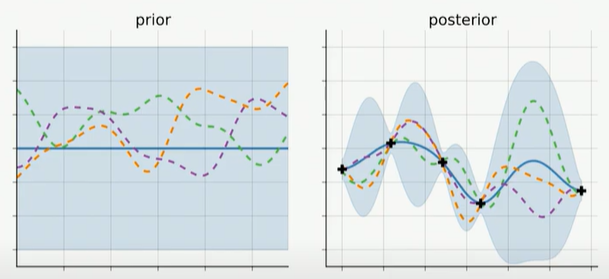
Our ultimate goal is to collapse the uncertainty surrounding the posterior mean of our model parameters in order to identify the best set of parameters. This is depicted in the figure2 below, where we reduce the blue-shaded area that represents our uncertainty regarding our parameterized model performance by repeatedly sampling and subsequently evaluating our surrogate models (dashed colored lines represented as Gaussian processes), and finally adjusting our surrogate models. (The mean of the Gaussian process represented as the solid blue line gives the approximate response)
 Each time we observe our function at a new point, this posterior distribution is updated.
Sequential model-based global optimization (SMBO)
In an application where the true function $f: \chi \rightarrow \mathbb{R}$ is costly to evaluate, model-based algorithms approximate $f$ with a surrogate that is cheaper. The point $x^*$ (in our case a set of hyperparameters) that maximizes the surrogate model becomes the proposal for where the true function should be evaluated.
[!info] SMBO iterates between fitting models and using them to make choices about which configurations to investigate. It offers the appealing prospects of interpolating performance between observed parameter settings and of extrapolating to previously unseen regions of parameter space. It can also be used to quantify importance of each parameter and parameter interactions.
The psuedo-code for how SMBO algorithms model $f$ via observational history $\mathcal{H}$ is as follows:
\begin{algorithm}
\caption{SMBO}
\begin{algorithmic}
\PROCEDURE{SMBO}{$f, M, T, S$}
\STATE $ \mathcal{H}\leftarrow \phi $
\FOR{$t \leftarrow 1 \; to \; T$}
\STATE $ x^* \leftarrow  \underset{x}{argmin} \; S(x, M_{t-1}) $
\STATE $\text{EVALUATE} \; f(x^*) $
\STATE $\mathcal{H}\leftarrow \mathcal{H} \cup (x^*, f(x^*))$
\STATE $\text{ fit a new model} \; M_t \; \text{to} \; \mathcal{H}$
\ENDFOR
\RETURN $\mathcal{H}$
\ENDPROCEDURE
\end{algorithmic}
\end{algorithm}
A probabilistic surrogate model
SMBO algorithms differ in what criterion they optimize to obtain $x^*$ given a surrogate of $f$. The novel work of Bergstra et al. proposed creating a probabilistic surrogate model of $f$ by modeling a hierarchical Gaussian process, and use expected improvement (EI) as the acquisition function. In their case, they implement EI via a tree-structed Parzen estimator (TPE).3 The processes can be written as follows:
\begin{algorithm}
\caption{BO}
\begin{algorithmic}
\PROCEDURE{BO}{$f, n, T$}
\STATE $\text{Place a Gaussian process prior on objective function} \; f$
\STATE $\text{Observe} \; f \; \text{at} \; n \; \text{points according to an initial space-filling experimental design}$
\FOR{$t \leftarrow 1 \; to \; T$}
\STATE $\text{Update the posterior probability distribution of} \; f \; \text{using all available data}$
\STATE $\text{Calculate the maximizer of the acquisition function to find the next sampling point}$
\STATE $x_t^* = \underset{x}{argmax} \; Acquisition(x|\mathcal{D}_{1:t-1})$
\STATE $\text{Pass the parameters to the objective function to obtain a sample}$
\STATE $y_t= f(x_t^*)$
\STATE $\text{Add sample to previous samples}$
\STATE $\mathcal{D}_{1:t} = \mathcal{D}_{1:t-1}, (x_{t} ,y_t)$
\ENDFOR
\RETURN $\mathcal{H} \vdash \; \underset{\mathcal{H}}{argmin} \; y$
\ENDPROCEDURE
\end{algorithmic}
\end{algorithm}
The EI acquisition function that we will optimize to choose the next experiment can be represented as follows:
Here $x$ is our set of hyperparameters, $y^{}$ is our target performance/value of the best sample so far, and $y$ is our loss. We want the $p(y < y^{})$, which we will define using a quantile search result to achieve the following:
| Most other surrogate models like Random Forest Regressions and Gaussian-processes represent $ p(y | x) $ like in the EI equation above, where $y$ is the value on the response surface, i.e. the validation loss, and $x$ is the hyper-parameter. However, TPE calculates $p(x | y)$ which is the probability of the hyperparameters given the score on the objective function. This is done by replacing the distribution of the configuration prior with non-parametric densities. The TPE defines $p(x | y)$ using the following two densities: |
The explanation of this equation is that we make two different distributions for the hyperparameters: one where the value of the objective function is less than a threshold $y^{}$, $l(x)$, and one where the value of the objective function is greater than the threshold $y^{}$, $g(x)$. In other words, we split the observations in two groups: the best performing one (e.g. the upper quartile) and the rest, defining $y^*$ as the splitting value for the two groups (often represented as a quantile).
After constructing two probability distributions for the number of estimators, we model the likelihood probability for being in each of these groups (Gaussian processes to model the posterior probability). Ultimately we want to draw values of x from l(x) and not from g(x) because this distribution is based only on values of x that yielded lower scores than the threshold. Interestingly, Bergstra et al. show that the expected improvement is proportional to $\frac{l(x)}{g(x)}$, so we should seek to maximize this ratio.
Putting the above together, our surrogate modeling process looks like the following:
- Draw sample hyperparameters form $l(x)$
- Evaluate the hyperparameters in terms of $\frac{l(x)}{g(x)}$
- Return the set of hyperparameters that yields the highest value under $\frac{l(x)}{g(x)}$
- Evaluate these hyperparameters via the objective function
If the surrogate function is correct, then these hyperparameters should yield a better value when evaluated.
A bit more on TPEs
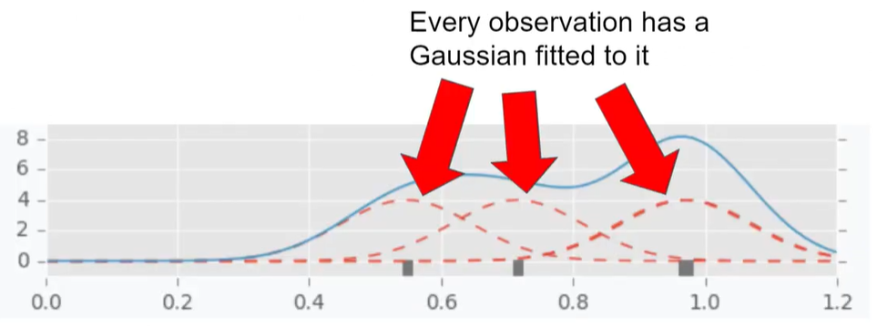
The two densities l and g are modeled using Parzen estimators (also known as kernel density estimators) which are a simple average of kernels centered on existing data points. In other words, we approximate our PDF by a mixture of continuous distributions. This is useful since we assume that there is some unknown but nonzero density around the near neighborhood of $x_i$ points and we use kernels $k$ to account for it. The more points is in some neighborhood, the more density is accumulated around this region and so, the higher the overall density of our function. For example, below4 we have a density displayed via the blue line which could represent $l$ or $g$, and three observations with Gaussian kernels centered on each.

To see how likely a new point is under our mixed distribution, we compute the mixture probability density at a given point $x_i$ as follows:
.
Implementation
Lets use this function for our objective function:
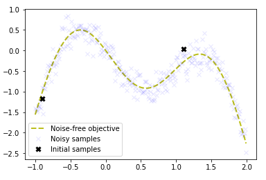
The following plot shows the noise-free objective function, the amount of noise by plotting a large number of samples and the two initial samples.

We are trying to find the global maximum at the left peak, via the fewest number of steps. Now we will implement the acquisition function defined as the expected improvement function above.
def ei_acquisition(X, X_sample, Y_sample, gauss, xi=0.01):
    """
    Expected improvement at points X using Gaussian surrogate model
    """
    mu, sigma = gauss.predict(X, return_std=True)
    mu_sample = gauss.predict(X_sample)

    sigma = sigma.reshape(-1, 1)

    mu_sample_opt = np.max(mu_sample)

    with np.errstate(divide='warn'):
        imp = mu - mu_sample_opt - xi
        Z = imp / sigma
        ei = imp * norm.cdf(Z) + sigma * norm.pdf(Z)
        ei[sigma == 0.0] = 0.0

    return ei


def min_obj(X):
    # Minimization objective is the negative acquisition function
    return -ei_acquisition(X.reshape(-1, dim), X_sample, Y_sample, gauss)
Now we are ready to run our experiment:

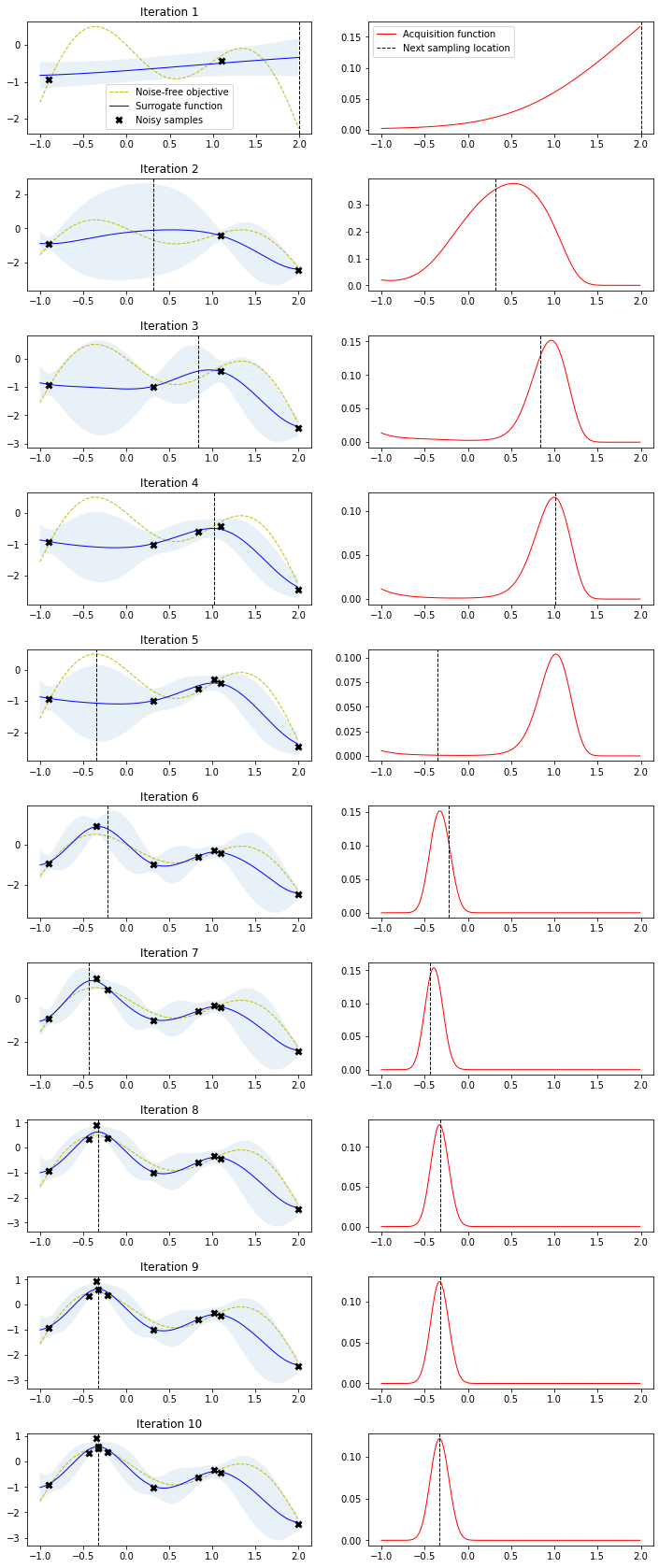
Bayesian optimization runs for 10 iterations. In each iteration, a row with two plots is produced. The left plot shows the noise-free objective function, the surrogate function which is the GP posterior predictive mean, the 95% confidence interval of the mean and the noisy samples obtained from the objective function so far. The right plot shows the acquisition function. The vertical dashed line in both plots shows the proposed sampling point for the next iteration which corresponds to the maximum of the acquisition function.
Note how the two initial samples initially drive search into the direction of the local maximum on the right side but exploration allows the algorithm to escape from that local optimum and find the global optimum on the left side. Also note how sampling point proposals often fall within regions of high uncertainty (exploration) and are not only driven by the highest surrogate function values (exploitation).
A convergence plot reveals how many iterations are needed the find a maximum and if the sampling point proposals stay around that maximum i.e. converge to small proposal differences between consecutive steps.

[!danger] Bayesian optimization is efficient in tuning few hyper-parameters but its efficiency degrades a lot when the search dimension increases too much, up to a point where it is on par with random search.
-
Bergstra, James & Bengio, Y.. (2012). Random Search for Hyper-Parameter Optimization. The Journal of Machine Learning Research. 13. 281-305. ↩
-
Rasmussen & Williams, Gaussian Processes for Machine Learning, MIT Press 2006. ↩
-
James Bergstra, Rémi Bardenet, Yoshua Bengio, and Balázs Kégl. 2011. Algorithms for hyper-parameter optimization. In Proceedings of the 24th International Conference on Neural Information Processing Systems (NIPS’11): 2546–2554. ↩
-
https://www.youtube.com/watch?v=bcy6A57jAwI&t=620s ↩