Probabilistic Generative Models- Normalizing Flows
Introduction
Both GAN and VAE lack the exact evaluation and inference of the probability distribution, which often results in low-quality blur results in VAEs and challenging GAN training in GANs with challenges such as mode collapse and vanishing gradients posterior collapse, etc. VAEs specifically can sometimes suffer from blurry or incomplete reconstructions due to the limitations of the variational inference framework. This is because due to the complexity of real-world data distributions, the mapping from the latent space to the data space may not cover the entire data space, leading to incomplete coverage and potentially missing regions of the target distribution.
Normalizing flows were proposed to solve many of the current issues with GANs and VAEs by using reversible functions to explicitly model the mapping from the latent space to the data space without relying on an approximation. The main idea is to learn a mapping from a simple distribution to a target distribution by composing a sequence of invertible transformations, where each transformation is itself an invertible neural network. By applying these transformations, the model can learn to capture the complex dependencies and multimodal nature of the target distribution.
Mathematical Prerequisites
Change of variables:
where:
- $p_x(x)$ is the density of $x$
- $p_z(x)$ is the density of $z$$ - our latent distribution
- $f(x)$ is an invertible, differentiable transformation
-
$ \text{det}Df(x) $ is a volume correction term that ensures that $x$ and $z$ are valid probability measures (integrate to 1)1 - $Df(x)$ is the Jacobian of $f(x)$
Ex.

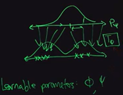
Ultimately, we want to find a $p_z(x)$ that is easy to work with, by finding the function that transforms the complex distribution $p_x(x)$ (our data) into $p_z(x)$. So for example, making the distribution of our images $p_x(x)$ look like Gaussian noise.
Where Normalizing Flows Comes In
Normalizing flows says that given eq. 1, we want to find the $f(x)$, which is our flow. Our base measure $p_z(x)$ is typically selected as $N(z|0, I)$, hence the normalizing in normalizing flows. So if we can find $f(x)$ that gets us from $p_x(x)$ to $p_z(x)$, then we can perform the two tasks vital for PGMs:
- Sample- $z \sim p_z(\cdot)$
- Evaluate\compute $x = f^{-1}(z)$
We train the NF by maximum (log-) likelihood:
| where $\theta$ are the parameters of the flow $f(x | \theta)$. It is constructing these flows that is the key research problem with NFs. |

In terms of notation in the above sketch, we want to learn the parameters of $T_\phi$ that achieve the bijective mapping.
TLDR: Find the parameters of the normalizing flow that best explains our data, by maximizing the likelihood of observing our data given those parameters
| This can also be thought of as minimizing the KL divergence between $p_x(x)$ and $p_z(x)$. Similar to our approach in VAE, we can evaluate $KL((p_z(x) | (p_x(x)))$ as $=\text{const.} - \mathbb{E}_{x\sim p_z(x)}[\text{log}p_x(x)]$. If we replace $p_x(x)$ in the expectation, we get eq. 2 above! |
This is the advantage with normalizing flows:
[!Takeaway] We can sample from the base measure ($z$), push it through the transform (flows) $f$, and then minimize the KL divergence like we do with VAEs but it a more differentiable way.
More on the Flows
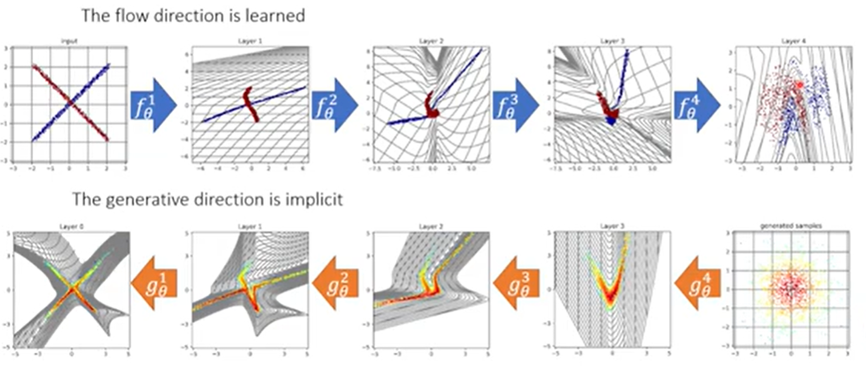
Instead of a single flow $f(x)$, we are going to use a composition of flows. We can do this since invertible, differentiable functions are closed under composition2:
This allows us to build a complex flow from the composition of simpler flows. This is similar to stacking layers in a DNN.
![Source: [^1]](/My-DS-Blog/images/NF_flows.png)
This means that the determinant term in eq. 1 and eq. 2 can now be expressed as the product of the determinants of the individual functions:
So now we can rewrite eq. 2 as:
Coupling Flows
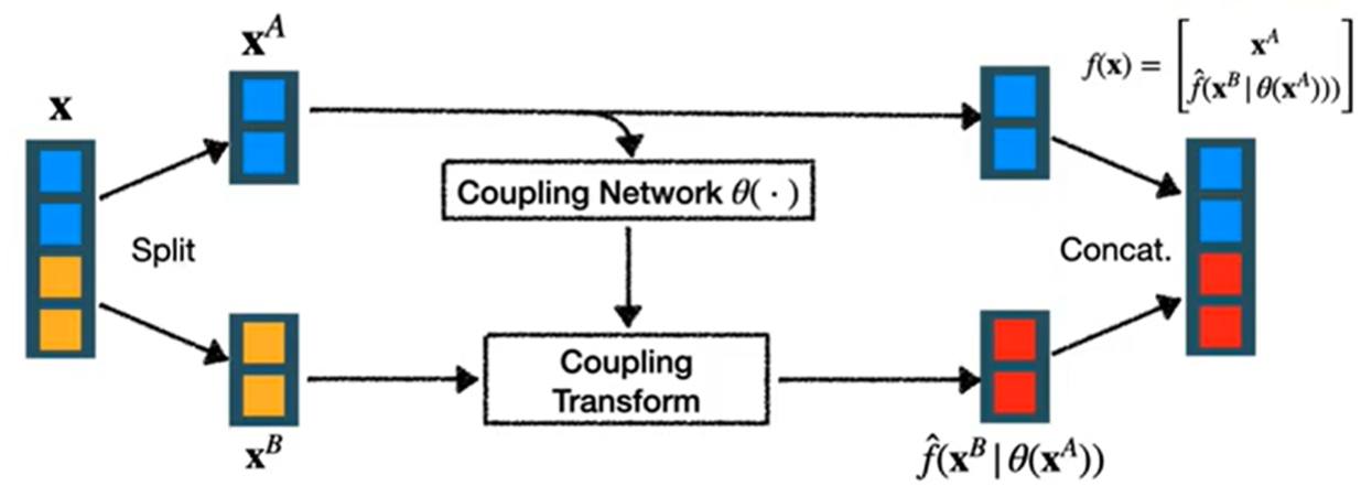
We use coupling flows as a general approach to construct non-linear flows. We partition the parameters into two disjoint subsets $x = (x^A, x^B)$ then
| where $\hat{f}(x^B | \theta(x^A))$ is another flow but whose parameters depend on $x^A$. |
Forward- the flow direction

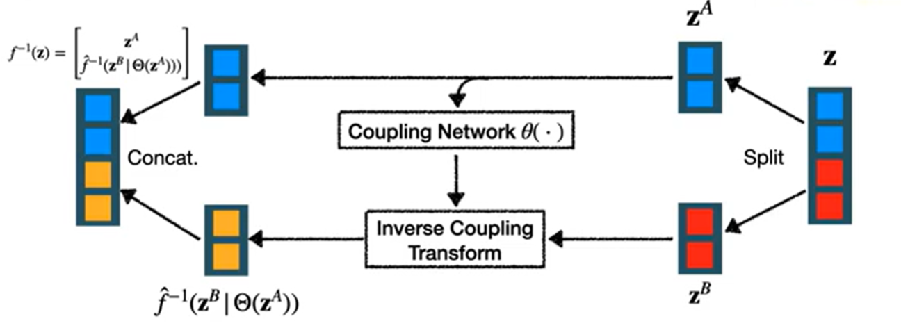
The $\theta$ in the coupling network above can be an arbitrarily complex function, like a MLP, CNN, etc. The parameters output from the coupling network are then applied to the second split in what is labeled as the coupling transform above.
For example, if $f$ is a linear transformation (an affine flow), the coupling network learns $s$ and $t$ to represent scale and translation using $x^A$. Then $f$ applies to $x^B$ using $s, t$ would look like $s \cdot x^B + t$.
We repeat this splitting process, applying shuffling, and go around and around until each part of $x$ has a chance to be a part of the conditioning coupling network.
Inverse: the generative direction

Training Process
- Get a example from the dataset $x$
- Flow to $z$ space $z=f_\theta(x)$
-
Account for change in probability mass by calculating the determinant of the Jacobian $\text{log} \text{det}Df_\theta(x) $ which for the affine flow is just the determine of the scale $\sum\text{log} s $ -
Calculate the loss: $L = z _2^2 + \sum\text{log} z $ - Update $\theta$

-
The determinant of the Jacobian matrix encapsulates how a function distorts or stretches the local space around a point. It quantifies the local scaling factor and provides information about orientation preservation or reversal. If it is large, it means that the transformation significantly stretches or shrinks the local space, given a measure of local scaling. The sign of the determinant tells us whether the transformation preserves or reverses the orientation of the local space. ↩
-
Function composition is a way of combining two functions to create a new function by applying one function to the output of the other function. A set or collection of objects is said to be closed under a certain operation if applying that operation to any two objects in the set always produces another object that is also in the set. For example, consider a set of functions S. We say that this set of functions is closed under composition if, for any two functions f and g in S, the composition of f and g, denoted as f(g(x)), is also in S. ↩